
 Tweet
Tweet
This might not settle it but it sure has some interesting info. Note the last comment that the only thing that separates A. Peterson from the rest of the RBs is 2% of the runs. I think the same analogy applies to FWP. (Hmmm, the biologists tell us the only thing separating us from the monkeys is 2% of our DNA......) Anyway, do we want a boom and bust guy or steady-eddie? The answer is....it depends:
Comparing Running Performance
This post follows a discussion of how to rate running back performance (or team rushing performance) that began at PFR and continued at Smart Football. I'll add my two cents here.
Yards per carry (YPC) is a useful stat, but it doesn't tell us everything we want to know. Median yards gained isn't very useful because, with rare exceptions, every RB will have a median gain of 3 yds. There are any number of suggestions for alternate measures such as yards above team median, yards above replacement, or success rate (the Hidden Game of Football system used by Football Outsiders). The comments at the Smart Football post feature a great discussion of the topic. Unfortunately, there really is no single number that can capture the full picture. In fact, what we really need is a picture.
I'll explain that in a minute, but first I want to address an age-old water cooler question that Chris discussed in his post at Smart Football. Consider two RBs, both with identical YPC averages. One however, is a boom and bust guy like Barry Sanders, and the other is a steady plodder like Jerome Bettis. Which kind of RB would you rather have on your team?
The answer is it depends. Essentially, we have a choice between a high-variance RB and a low-variance RB. When a team is an underdog, it wants high-variance intermediate outcomes to maximize its chances of winning. And when a team is a favorite, it wants low-variance outcomes. Whether those outcomes occur through play selection, through 4th down doctrine, or through RB style isn't important. If you're an otherwise below-average team, you'd want the boom and bust style RB. If you're an otherwise above-average team, you'd want the steady plodder.
The same concept applies within a game. If you're losing during a game, you have become the underdog no matter how strong your team seemed on paper before kickoff. In this case, you want to increase the risk-reward balance with high-variance plays. You'd accept the risk of a 10-yd loss in the backfield for the possibility of breaking a 40-yd run. But if your team is up by a TD, the 10-yd loss isn't so acceptable.
Further, even if the high-variance RB has a lower average YPC, we'd still might want him carrying the ball when we're losing. This is due to the math involved in competing probability distributions.
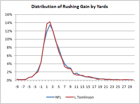
Now back to the question on how to evaluate a RB or team rushing game. Mean, median, or even mode are handy ways of describing a central tendency. But on their own, they don't paint the whole picture. It's a bit like the proverb about several blind men each grasping a part of an elephant. We could say that LaDainian Tomlinson's 4.4 career YPC figure is good because it's above average, but it doesn't tell us much more than that. It's like grasping the elephant's trunk. Instead, we can look at the whole elephant.
Below is the distribution of Tomlinson's career gains. The horizontal axis are the gains, and the vertical axis represents how often he got each gain. The blue line is distribution for the NFL as a whole, and the red line is Tomlison's distribution.
We could simplify the distribution into large bins selected for certain signifcance. For example, we could divide the distribution into all losses, gains of 1-4 yds, 5-10 yds, and 10 yds or more. Tomlinson might be a "10/45/35/10." This is unwieldy, but it's not much different than how the baseball guys use a similar shorthand for wOBA, BAPIP, and the other stats they often bundle together.
Not that I'd ever expect anyone to use this, but we could use a more technical shorthand. The RB gain distributions can be modeled as a gamma distribution, a bell-type curve described by 2 parameters--k and theta. For example, Tomlinson is a Gamma(11, 1.1). That's about all we'd need to know to reproduce his gain distribution. The parameters are not intuitive at all, so it's not a workable solution. (Perhaps someone out there might suggest a better type of distribution to use.)
To be honest, I was expecting a bigger difference between Tomlinson and the rest of the league. So I looked at some other RB's distributions. I wanted to see a difference between boom-and-bust guys and plodder-types. I picked Adrian Peterson and Brian Westbrook to compare to Jerome Bettis and Jamal Lewis. Their distributions are plotted below.

What amazes me is how similar they all are to each other and to the league average. One notable exception is Jamal Lewis' peak. He has significantly more runs of between 0 and 3 yards than other backs. If you read the plot the wrong way, this might appear good, but it's defninitely not. Usually, a RB needs 4 to 5 yards to just break even in terms of his team's probability of converting a first down. What we'd want to see on a RB's distribution is as much probability mass as possible to the right of 4 yards.
So if Bettis' distribution looks so much like Tomlinson's, how does Bettis have a 3.9 career YPC and Tomlinson have a 4.4 career YPC? As others have noted previously, the difference among RB YPC numbers primarily come from big runs. It's the open field breakaway ability that separates the guys with big YPC stats from the other RBs. Of Tomlinson's runs, 1.5% were for 30 yards or more. Bettis' 30+ yd gains comprised only 0.46% of his carries. The other RBs and the league average are as follows:
NFL 0.91%
Lewis 0.88%
Westbrook 0.93%
Peterson 2.20%
Adrian Peterson's 2.2% figure is exceptional. It's interesting because it really suggests that what separates Peterson as a great runner is based on only 2% or so of his runs. Otherwise, he's practically average.
Of course, the usual caveats apply. When talking about a specific RB, we are really talking about his team's running performance when the RB has the ball. And we haven't considered game situation yet. Ideally, we'd want to plot a series of distributions, one for each typical down and distance situation--1st and 10, 2nd and long, 2nd and mid/short, and 3rd and short. But that's a far cry from a nice handy single number.
[url]http://www.advancednflstats.com/2009/08/comparing-running-performance.html[/url]
Comparing Running Performance
This post follows a discussion of how to rate running back performance (or team rushing performance) that began at PFR and continued at Smart Football. I'll add my two cents here.
Yards per carry (YPC) is a useful stat, but it doesn't tell us everything we want to know. Median yards gained isn't very useful because, with rare exceptions, every RB will have a median gain of 3 yds. There are any number of suggestions for alternate measures such as yards above team median, yards above replacement, or success rate (the Hidden Game of Football system used by Football Outsiders). The comments at the Smart Football post feature a great discussion of the topic. Unfortunately, there really is no single number that can capture the full picture. In fact, what we really need is a picture.
I'll explain that in a minute, but first I want to address an age-old water cooler question that Chris discussed in his post at Smart Football. Consider two RBs, both with identical YPC averages. One however, is a boom and bust guy like Barry Sanders, and the other is a steady plodder like Jerome Bettis. Which kind of RB would you rather have on your team?
The answer is it depends. Essentially, we have a choice between a high-variance RB and a low-variance RB. When a team is an underdog, it wants high-variance intermediate outcomes to maximize its chances of winning. And when a team is a favorite, it wants low-variance outcomes. Whether those outcomes occur through play selection, through 4th down doctrine, or through RB style isn't important. If you're an otherwise below-average team, you'd want the boom and bust style RB. If you're an otherwise above-average team, you'd want the steady plodder.
The same concept applies within a game. If you're losing during a game, you have become the underdog no matter how strong your team seemed on paper before kickoff. In this case, you want to increase the risk-reward balance with high-variance plays. You'd accept the risk of a 10-yd loss in the backfield for the possibility of breaking a 40-yd run. But if your team is up by a TD, the 10-yd loss isn't so acceptable.
Further, even if the high-variance RB has a lower average YPC, we'd still might want him carrying the ball when we're losing. This is due to the math involved in competing probability distributions.
Now back to the question on how to evaluate a RB or team rushing game. Mean, median, or even mode are handy ways of describing a central tendency. But on their own, they don't paint the whole picture. It's a bit like the proverb about several blind men each grasping a part of an elephant. We could say that LaDainian Tomlinson's 4.4 career YPC figure is good because it's above average, but it doesn't tell us much more than that. It's like grasping the elephant's trunk. Instead, we can look at the whole elephant.
Below is the distribution of Tomlinson's career gains. The horizontal axis are the gains, and the vertical axis represents how often he got each gain. The blue line is distribution for the NFL as a whole, and the red line is Tomlison's distribution.
We could simplify the distribution into large bins selected for certain signifcance. For example, we could divide the distribution into all losses, gains of 1-4 yds, 5-10 yds, and 10 yds or more. Tomlinson might be a "10/45/35/10." This is unwieldy, but it's not much different than how the baseball guys use a similar shorthand for wOBA, BAPIP, and the other stats they often bundle together.
Not that I'd ever expect anyone to use this, but we could use a more technical shorthand. The RB gain distributions can be modeled as a gamma distribution, a bell-type curve described by 2 parameters--k and theta. For example, Tomlinson is a Gamma(11, 1.1). That's about all we'd need to know to reproduce his gain distribution. The parameters are not intuitive at all, so it's not a workable solution. (Perhaps someone out there might suggest a better type of distribution to use.)
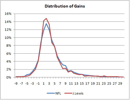
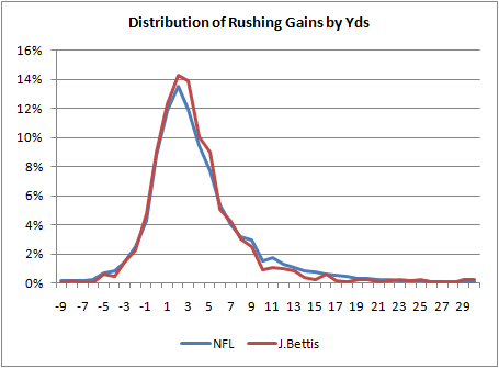
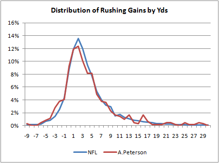
To be honest, I was expecting a bigger difference between Tomlinson and the rest of the league. So I looked at some other RB's distributions. I wanted to see a difference between boom-and-bust guys and plodder-types. I picked Adrian Peterson and Brian Westbrook to compare to Jerome Bettis and Jamal Lewis. Their distributions are plotted below.
What amazes me is how similar they all are to each other and to the league average. One notable exception is Jamal Lewis' peak. He has significantly more runs of between 0 and 3 yards than other backs. If you read the plot the wrong way, this might appear good, but it's defninitely not. Usually, a RB needs 4 to 5 yards to just break even in terms of his team's probability of converting a first down. What we'd want to see on a RB's distribution is as much probability mass as possible to the right of 4 yards.
So if Bettis' distribution looks so much like Tomlinson's, how does Bettis have a 3.9 career YPC and Tomlinson have a 4.4 career YPC? As others have noted previously, the difference among RB YPC numbers primarily come from big runs. It's the open field breakaway ability that separates the guys with big YPC stats from the other RBs. Of Tomlinson's runs, 1.5% were for 30 yards or more. Bettis' 30+ yd gains comprised only 0.46% of his carries. The other RBs and the league average are as follows:
NFL 0.91%
Lewis 0.88%
Westbrook 0.93%
Peterson 2.20%
Adrian Peterson's 2.2% figure is exceptional. It's interesting because it really suggests that what separates Peterson as a great runner is based on only 2% or so of his runs. Otherwise, he's practically average.
Of course, the usual caveats apply. When talking about a specific RB, we are really talking about his team's running performance when the RB has the ball. And we haven't considered game situation yet. Ideally, we'd want to plot a series of distributions, one for each typical down and distance situation--1st and 10, 2nd and long, 2nd and mid/short, and 3rd and short. But that's a far cry from a nice handy single number.
[url]http://www.advancednflstats.com/2009/08/comparing-running-performance.html[/url]

Comment